In presenting the theory, I struggled with whether it was best to introduce the rules and application of the theory or introduce the original mapping concept I presented as an undergraduate. After discussing this with several colleagues, I decided to share the original concept as a starting point. It is, after all, where it begins for me.
By mentally placing myself in the early nineteen hundred and imagining reading an experiment that showed a clock ran at a different rate high on a mountain than it did in the valley, how would I have perceived it? My initial thought (after listening to colleagues of the time and considering how they came to their conclusion) is that gravitational potential plays a role in determining the clock’s rate. From this idea, I developed a conceptual map of space about a massive body. And evaluate its competence by comparing it to empirical data.
Since the clock appeared to dilate by a scalar factor, I knew whatever mapping of a field about a massive object was, it would be a scalar for this measurement. If it was based on gravitational potential energy, then the potential needed to be divided by another energy to form a unitless scalar (or the gravitational potential was to be the divisor of another energy). The obvious question was, what energy? To answer this question, one must go back to my original thought that led me to college and ultimately write this book. That thought was that space produces the energy needed to maintain the physical world as we know it. And if it produces the energy, then space can have places of differing energy available for maintaining the physical world. Now, it is not to be discussed here whether or not this original idea is valid. What is to be drawn from it is this is the thought that inspired me to take this journey. Thus, it was natural from my thought process to imagine the rest mass energy of SR that was to be introduced as the secondary energy used in mapping space about a massive object. Therefore, I tried dividing the gravitational potential by the rest of the energy of the mass generating the potential and evaluating how it compares to the scaled time dilation at different elevations.
One problem arose instantly when I jotted it down on paper. To calculate the gravitational potential energy, one needs two masses since Newtonian gravitational potential energy is defined as
$$
\begin{equation}\label{eqNewtonianGravitationalPotential}
V = \frac{G M_1 M_2}{r}
\end{equation}$$
where \(V\) is the gravitational potential, \(G\) is the Newtonian gravitational constant, \(M_1\) and \(M_2\) are masses, and \(r\) is the radial distance between the centers of the two masses.
Mapping the scenario, there is only one mass generating the gravitational field. As an undergrad, I pondered on this for a while; I didn’t like the idea of a test mass, and if one used an arbitrary mass, the scalar would not be invariant between observers. I questioned, what if the mass generating the potential was moved an infinite distance away under its own influence? This led me to the concept of a virtual mass (of course, I also thought as an undergrad that if quantum can use virtual particles, gravity can use virtual masses). The concept is straightforward: the first mass is the physical mass generating the gravitational field, and the second mass is a virtual point mass of equal magnitude to the generating mass. A virtual mass would be placed at every location in space about the generating mass. Then, a gravitational potential-based field is derived. This potential would then be divided by the rest energy of the generating mass. Thus providing a NUVO transformational derived potential of:
$$\begin{equationblock}{NUVO Transformation Potential}
\begin{equation}\label{eqNUVOGravitationalPotential}
V_g = \frac{G M_1 M_v}{r}
\end{equation}
\end{equationblock}$$
$$\begin{equation} \label{eqNUVOTranformationGravitationalPotential}
\phi = \frac{V_g}{M_1 c^2}=\frac{G M_v}{r c^2}
\end{equation}$$
The second postulate of Einstein’s Special Relativity states the speed of light is constant for all observers in an inertial frame, independent of the motion of the emitting body. Maintaining this postulate and constraining any metric to require $\hat{x}=c \hat{t}$ then the following relations hold.
\begin{equation}\label{eqRelation1}
c = \frac{\hat{x}}{\hat{t}} \rightarrow \hat{x} = c \hat{t} \rightarrow \hat{t} = \frac{\hat{x}}{c}
\end{equation}
Equation above implies if length (\(\hat{x}\)) expands or contracts, then so must time (\(\hat{t}\)) expand or contract respectively. Thus, if length transforms by \(\phi\), then time must transform by the same value. The following transformation is applied when the time component is transformed:
\begin{equationblock}{NUVO Time Transformation}
\begin{equation}\label{eqTimeTransformation}
t_g = \frac{G M_1 M_v}{c t} = \frac{G M_1 M_v}{r}
\end{equation}
\end{equationblock}
Thus, the transformation at this point in the development has two parameters: Potential for change in length (\(V_g\)) and change in time (\(t_g\)). \(\Phi\) now takes the form of:
\begin{equation} \label{eq:4.6}
\phi = \frac{V_g +t_g}{M_1 c^2} =\frac{G M_v}{r c^2}+\frac{G M_v}{c\: t\: c^2} = \frac{2 G M_v}{r c^2}
\end{equation}
If there is no change in position \(r\), then \(V_g\) is zero, same with \(t_g\); if there is no change in time, then \(t_g\) is zero. This transformation provides a path for a ratio of the virtual gravitational potential energy at a location to the rest energy of the mass generating the potential to be applied. This obviously didn’t match empirical data, but quickly (in one setting), I discovered if you add it to one and assign a scalar value (as equated at a location) to the location on top of the mountain and assigned a scalar value to the location in the valley and take their difference, it matched the empirical data with one exception, the clock rates were reversed (the clock on the mountain had a “longer” tick than the one in the valley). None-The-Less is one surprise I had in my journey; my original idea while watching a documentary produced actual results.
\begin{equation}
\begin{split}
\phi_{mountain} = 1 + \frac{V_g + t_g}{E_0} = 1 + \frac{G M_v}{r_{mountain}c^2} \
\phi_{valley} = 1 + \frac{V_g + t_g}{E_0} = 1 + \frac{G M_v}{r_{valley}c^2} \
\Delta t = \phi_{mountain} -\phi_{valley}
\end{split}
\end{equation}
To correct the transformation to show the clock rates correctly, the inverse of \(\phi\) is used. Thus
\begin{equation}
\begin{split}
\phi_{mountain} = \frac{1}{1 + \frac{V_g + t_g}{E_0}} = \frac{1}{1 + \frac{G M_v}{r_{mountain}c^2}} \
\phi_{valley} = \frac{1}{1 + \frac{V_g + t_g}{E_0}} = \frac{1}{1 + \frac{G M_v}{r_{valley}c^2}} \
\Delta t = \phi_{mountain} -\phi_{valley}
\end{split}
\end{equation}
corrects the clock’s rate to match known data. This will be discussed later when Exemplar and Privo spaces are covered within the transformation.
Note \(t_g\) is zero since the measurements (one at the top of the mountain, the other at the bottom of the mountain) are made at the same time. Thus, there is no change in time between the measurements. Therefore, \(t_g\) is zero. This concept, when applied to the GPS system, matched the GR predicted dilation between the two locations. But it left me longing, as I desired a single transformation to represent both the GR and the miss-used SR effect as often used in explaining GPS time dilation. So, I pondered if the process of the division of gravitational potential energy by rest energy worked for the GR part, it might work for the kinetic part. Thus, I took the kinetic energy and divided it by the rest energy. The one constraint placed on the kinetic energy is the velocity within the kinetic energy portion of the transformation \textbf{must} be the instantaneous velocity because of acceleration. This is a distinguishing constraint that removes the ability to justify SR. Classical kinetic energy can
be shown as:
\begin{equation}
T =\frac{1}{2} M v^2
\end{equation}
Where \(v\) is the velocity of the mass, and M is the mass moving in the field.
Remember, there is a virtual mass mapping the field, and acceleration is required, thus the \(M\) in the kinetic equation is replaced with \(M_v\) and divided by the rest energy giving NUVO transformation derived value of:
\begin{equationblock}{NUVO Transformation Kinetic Energy \ (only use accelerated instantaneous velocity)}
\begin{equation}
T_g = M_v v^2
\end{equation}
\end{equationblock}
\begin{equation}\label{eqTransformation411}
\phi = 1 + \frac{T_g}{E_0} = 1 + \frac{M_v v^2}{2 M c^2}=1 + \frac{v^2}{2 c^2}
\end{equation}
From here it was rather trivial to arrive at a full scalar mapping for the field about the mass generating the field as a function of both NUVO transformational potential and NUVO transformational kinetic energy:
\begin{equationblock}{NUVO Transformation}
\begin{equation} \label{eqTransformation1}
\phi^{-1} = 1 + \frac{T_g + V_g + t_g}{E_0}
\end{equation}
\begin{equation}
\phi^{-1} = 1 + \frac{\sum_{}^{} T_g + \sum_{}^{} V_g + \sum_{}^{} t_g}{E_0}
\end{equation}
\end{equationblock}
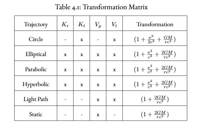
Transformation applies to a single mass. If there is more than one massive body interacting with a location in space, the sum of the \(V_g\) and \(t_g\) must be taken. \(T_g\) is because of acceleration and is a local effect. Thus, it is not a summation of global interacting bodies. Instead, it is a summation of kinetic in changing time and changing space. For instance, if a particle was orbiting about a central mass in a circle, there is no change in r (the radial distance), but there is a change in time as it orbits. Thus, \(T_g\) would be \(\frac{v^2}{2c^2}\), If it was an elliptical orbit, \(T_g\) would be \(2 \frac{v^2}{2c^2}\), a transformation for kinetic \textit{time} traversed, and kinetic \textit{distance} traversed.
Table below provides examples of transformations for different types of orbits. The circular orbit in the table is arguably non-existent in the physical world.
When two observers (observer A and B) are transforming measurements between their labs, the following transformation holds where $X_a$ represents a measurement by observer A in A’s frame:
\begin{equationblock}{Application of the NUVO transformation between two observers (A and B). Identity}
\begin{equation} \label{eqTransformation2}
\phi_a X_a = \phi_b X_b
\end{equation}
Which leads to
\begin{equation}\label{eqTransformation3}
X_a = \frac{\phi_b}{\phi_a} X_b
\end{equation}
\end{equationblock}
This is the formed I used in my undergrad presentation. This mapping predicted the GPS time dilation and Mercury’s perihelion advance. It also predicted there was a constant (invariant) length advance for any orbit about a mass. For instance, in our solar system, the advance in meters of Mercury is equal (to first order) to the advance in meters of Earth (or any other orbiting body about the sun). It is a universal constant for the system. It differs from system to system depending on the central mass, but it is constant for the system. One may say wait, that is not correct, Mercury’s advance is much more pronounced than Earth’s. I agree, but the advance in meters is the same (again to first order, which still makes them nearly equal). The ratio of advance in meters (approximately 29,000 meters) to the orbital circumference of Mercury is much more pronounced than the same advance in meters to the orbital circumference of the Earth.
With this scalar mapping, the main NUVO transformation is derived. Sadly it took over 10 years (as life happens) to realize this as the main NUVO transformation. Again, it originated from the concept that space provides the maintaining energy for all physical matter, and space has a finite amount of energy.
Here the concept of Exemplar \(\mathcal{E}\) and Privo \(\mathcal{P}\) space originate. Calculating the value of \(\phi\) equates to 1 if and only if both \(T_g\) and \(V_g\) equal zero. The nice advantage of \(\phi =1\) becomes obvious mathematically. I would prefer to divide or multiply by one versus a decimal. Therefore a special name is given to a space where \(\phi = 1\), Exemplar space. In contrast, a space where \(\phi \neq 1\) is given a special name, Privo space, meaning it is degraded.
Note there is a necessity to use exemplar space in the transformation from one observer to another. This arises from the constraint an observer must make measurements in their local frame (their location). An observer is not privy to what the units of measurement (compared to their lab) are in the other lab. Thus, when transferring they need to only work with their measurements. This is where Exemplar space plays an important role; it is a space where all observers agree without having to be there to make a measurement. This will be more evident in the chapter discussing the rules of application.
The origin of the two spaces differs from NUVO’s given formal definition. As NUVO conceptual discussion progresses, it will be shown these spaces correspond to the two spaces (vacuum) coupling availability to matter. For now, it corresponds to how time dilation relates to gravitational potential and acceleration.