The curvature of a light ray was arguably the turning point for mainstream acceptance of Einstein’s General Relativity theory. When Sir Eddington successfully photographed the stars around the sun during an eclipse of the sun in 1919, the results matched Einstein’s prediction. Since that time, the curvature of light has been observed in many places, from our solar system to across the universe. It is a hallmark of Einstein’s theory. If this hallmark did not exist, this section would be equally appropriate in Volume 2 concerning the Quantum level results since photons also have a quantum behavior; it became apparent a plausible description of the path of the light ray is hyperbolic.
The logic behind the choice of hyperbolic curves arises from the observation (due to the NUVO transformation) that space expands (as previously discussed) when a trajectory travels from Exemplar to Privo. Since photons do not couple to space as massive particles do, they do not experience a local effect, only a global one. Therefore, the radial expansion in this trajectory is equivalent to the semi-major axis for a hyperbolic trajectory. The semi-minor axis is equivalent to the expansion plus the radius of the massive object (the semi-minor axis is the semi-major plus the radius of the massive object). This, in theory, allows the eccentricity of the hyperbolic trajectory to be a function of the radius of the massive object. This is possible since the expansion is a fixed amount for a mass, allowing the only dependency to be with the radial distance.
Please note: r is the Exemplar space observation, and “a” the semi-major axis, is the expansion magnitude.
An observer at distance r will emit a light ray path aimed at the edge of the massive body (distance R, the radius of the massive body). As the light ray travels toward the massive object, the surrounding space will expand by the length of the semi-major axis. This will cause the light to appear to bend around the massive object. Recall a photon is a massless particle, and by the definition of the model, it has zero pinertia. Therefore, there is no local effect of sinertia, only the global effect of the field’s gradient. Thus, the transformation of the photon’s trajectory is:
\begin{equation}
\phi^{-1}(r)_{\gamma}= \left( 1 + \frac{V_g + t_g}{E_0} \right) R =\left( 1 + \frac{2 G M}{R c^2} \right) R
\end{equation}
The photon follows a hyperbolic path, as shown below. The angle between the two lines with slope ±ab is the angle a photon’s path appears to bend around an object. Using the terms from the list blow with M equal to the mass of the sun and R equal to the radius of the sun, the model predicts a curvature of 1.752″ for a photon traveling closest to the surface of the sun. This is in good agreement with empirical data and GR’s prediction .
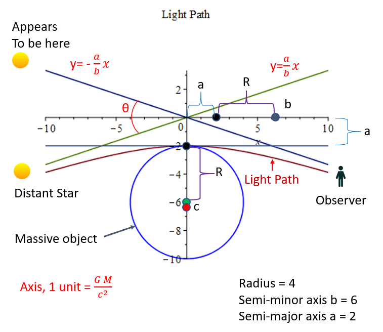
Light Ray Hyperbolic Path
- R = The radius of the massive body
- a = Semi-major axis a, with value (1+2GMRc2)R−R
- b = Semi-minor axis = R+a
- c = foci = a2+b2
- e = eccentricity = ca
- θ = arctan(2ab)
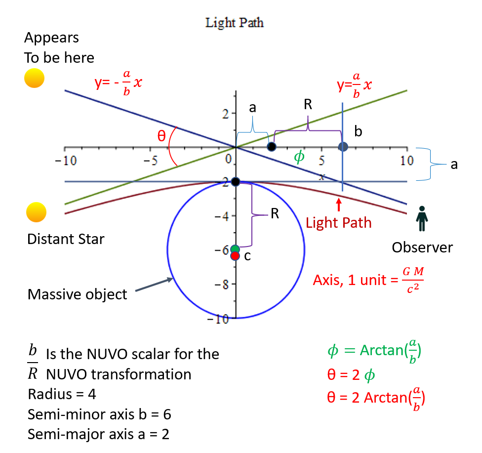
Note the values m1 and m2 are slopes of the asymptotic lines and not masses. This method can be applied to any distance from the central mass, not just its radius. Therefore, this method can predict the curvature of light about any massive body at any distance from the body. Note the NUVO transformation is reflected in the semi-minor axis of the hyperbola. The semi-major axis “a” represents the expansion in space, and “a” plus the radius R represents the observed radius from a distant observer. If one allows the mass to be considered a density over any radial distance, the value R can be interchanged with the distance “r” an observer is from the mass. In this scenario, the NUVO transformation scalar becomes br for an observer at distance r from the center of mass. The angle θ is 2tan−1(ab) and represents the total angle of displacement by a light ray traveling from a distant star to an observer on the opposite side of the massive object.
The unit value of length is set to GMc2, the characteristic length of the system as previously discussed. This can only be used when there is a single mass being considered or masses of equal magnitude. Otherwise, the value GMc2 will not be uniform, and a different unit value will need to be developed to plot a graph. Adding this information to the figure above one has the new figure below.
Consider:
\begin{equation}
x = r + a \end{equation}
\begin{equation}
\text{Divide by r}
\frac{x}{r} = 1 + \frac{a}{r}
\end{equation}
Substitute \(a\) value in to obtain
\begin{equation}
\frac{x}{r} = 1 + \frac{2 G M}{r c^2}
\end{equation}
Which is NUVO’s transformation Φ for a light path. The time and space dilation is simply the ratio of the Exemplar observed to the local Privo observed.
Note that the light path simplifies down to a function of expanding space. To calculate the angle of curvature about a mass at r distance, use the expansion (a) as such:
\begin{equation}
\theta = 2\left(\frac{a}{r_{exemplar}} \right)
\end{equation}
This is for weak fields. For strong fields, the more accurate arc tangent is applied
\begin{equation}
\theta = 2 tan^{-1}(\frac{a}{b})
\end{equation}
Where \(a\) is the semi-major axis and \(b\) is the semi-minor axis.
There is a logical path from the hyperbolic derivation of the light path to consider the NUVO transformation as
\begin{equation}\label{eqMasslessTransform1}
\phi = 1 + \frac{2 G M}{b c^2}
\end{equation}
Where \(r\) has been replaced with \(b\). Note \(b= R+a\); if this is the proper transformation to use, it allows \(R\), the radius of the mass, to go to zero, and the expansion of space is constant for the mass regardless of the radius. This concept is not applied to NUVO at the time of writing, but it is an area of investigation.