The math of General Relativity is based on differential geometry, specifically that of a Riemannian Manifold. Therefore, it would be ideal to start with this mathematical structure as an initial formalization. Einstein, in the beauty of his theory, gives a very simple-looking equation (though in the opinion of many, including the author, not simple in evaluation):
\begin{equation} \label{eqEinsteinGR}
R_{\mu \nu}-\frac{1}{2}R g_{\mu \nu} + \Lambda g_{\mu \nu}=\frac{8\pi G}{c^4}T_{\mu \nu}
\end{equation}
The simplicity of the concept is elegant. Stress energy warps space and the warping of space decides how a free particle moves. Arguably, the most popular solution to Einstein’s field equations is the Schwartzschild metric \cite{schwarzschild1999gravitational}. With this solution, one may solve for many of the predictions of GR, including the perihelion advance of Mercury (and other gravitational orbits), time dilation, light bending around massive objects, and so forth. Since the Schwartzschild metric is based on a static configuration (the field does not change over time), it does not directly support the calculations of gravitational waves, as they require the field to change over time as the wave propagates. Nonetheless, the Schwartzschild solution is elegant in the same manner as Einstein’s theory.
Although the NUVO transformation in a later chapter will be shown to be equivalent to a first-order series of Schwartzschild’s metric for time dilation, NUVO does not translate to a solution for Einstein’s field equations when one sets the stress-energy tensor equal to zero (empty vacuum). However, NUVO is not a solution to Einstein’s equations, which by itself doesn’t exclude the NUVO transformation from using the math structure of a manifold or possibly even a Riemannian manifold.
Another consideration is the local effect of NUVO. Einstein’s GR places an equal sign between the curvature of space-time and the energy. This curvature is of space-time, not a local effect. Thus, the momentum of the object is considered when calculating the curvature. In NUVO, this is separate; as such, the only way it can be a solution to Einstein’s field equations is if only the global is considered.
At this stage of development, the theory considers two events that dilate time in a field: the presence of a mass (globally affects the field) and the acceleration of mass (locally affects the field). Mass and energy in NUVO are not considered interchangeable globally; they are only between inertial frames, as in SR. Each of these will need to be treated separately and independently. Looking at the NUVO transformation, local and global effects are decoupled as:
\begin{equation} \label{eq9}
t_{\mathcal{P}}= \phi^{-1}(r)t_{\mathcal{E}} = \left[1 + \overbrace{ \frac{v^2_I}{2 c^2}}^\text{Local} + \overbrace{ \frac{G M}{r c^2}}^\text{Global} \: \right] t_{\mathcal{E}}
\end{equation}
The subscripts \(\mathcal{P}\) and \(\mathcal{E}\) are privo and exemplar space, respectively.
The kinetic energy contributes to the local part due to the acceleration of the particle moving in the field and, therefore, has a relative value to the frame from which it is observed. To standardize the observation, all measurements for the local part will be made locally with instantaneous velocity measured with respect to a stationary (in SR terms at rest) observer in \(\mathcal{E}\) space. In a configuration like the Schwartzschild metric, the central mass is at rest with an observer in \(\mathcal{E}\) space (at an infinite distance from the central mass), but caution should be used not to treat this as a default unless specified. In cases where the orbiting body’s mass is not much less than the central mass, a measurable effect may be lost by assuming the central mass is at rest (not moving) in relation to an observer at rest in \(\mathcal{E}\).
Armed with how to take measurements, the next step is to set up a manifold. The manifold \(\mathcal{M}\) is smooth with dimensions \(\mathcal{R}(3,1)\) with three spatial components and one temporal. The metric tensor is:
\begin{equation} \label{eqMetric}
g_{ij}=\phi(r) \: I
\end{equation}
Where \(I\) is the identity matrix, and \(\phi(r)\) is the NUVO transformation configured to evaluate both kinetic and potential on radial distance only. The metric reduces to a scalar ratio connection between local coordinate systems in an Euclidean coordinate system. Thus, a distance all observers agree to is:
\begin{equation} \label{eqDistance}
d^2=\phi(r)^{-2} \left( dx_1^2 + dx_2^2 + dx_3^2\right)
\end{equation}
Where the infinitesimal \(dx_i\) are measured locally. The time unit scales in the same manner as the length.
\begin{equation} \label{eqTime}
dt = \phi^{-1}(r) \: t
\end{equation}
Where unit time is measured locally.
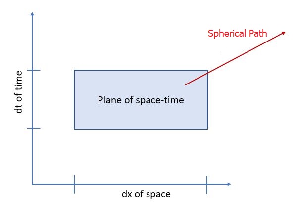
One observation from this configuration is one can form parallel tangent planes along the radial. On a spherical surface with a radius equal to the parallel planes tangent to the surface, all tangent spaces on the spherical surface will share the same scalar value for the metric. This is visualized in the figure below.

Further observation is as r→∞ the spherical surface asymptotically approaches the tangent surface. At an infinite distance from the massive object generating the field, the tangent and radial surfaces are the same. These infinitely distance tangent planes and radial surfaces correspond to E and have a ϕ(r) value of 1, allowing the entire space to be treated as Euclidean. As r→0, the rate at which the radial surface separates from the tangent plane (the curvature) increases. For now, dealing with the point at r=0 is delayed until later in the formalization for reasons that will become apparent.
A foliation of manifolds formed by concentric spheres where 0<r≤∞ is formed. Each manifold will have the same scalar-valued metric for the entire surface. Transforming coordinate values from one leaf of the foliation to another amounts to a scalar multiple of the coordinates. In this transformation, consider the following calculation. Pick any r value greater than zero and not in E and draw out a great circle path on the sphere’s surface with radius r. Align a plane such that it contains the great circle path. On the plane, it will form a circle of radius r′ as measured locally. Project this circle onto a parallel plane in E, and it will form a circle with a radius less than r′. This can be shown by applying the NUVO transformation and transferring the length of radius r′ to E. The reverse process can be performed by using the inverse of ϕ(r), in which case the image of the circle in E will be projected onto a leaf in P space.
Next, consider a test particle moving along this path and how its trajectory is transferred to the plane in E. This requires the local effect to be considered in addition to the global effect since the trajectory must have a velocity about the path to traverse the path. Here, the dimensions of 3+1 come into play. Unlike GR, this is three dimensions with time separate; thus, the distance does not include time in its calculation. Nonetheless, time is being swept out as the test particle transverses the path, and as such, its transformation scalar from ϕ(r) should be considered. To visualize, see the figure below as space is traversed, so is time; therefore, the value of ϕ(r) should be included when moving through time and space.
Thus, a particle undergoing acceleration will traverse an arc length greater than the arc length predicted by the calculation using only the global effects of the field. Both indicate a greater arc length than if there is no field effect (global or local). The local effect is predicted for both a gravitation field generated by a mass and in an empty vacuum. Consider only the gravitational field (global):
\begin{equation} \label{eq10}
2\pi r_{\mathcal{P}}= 2 \pi \phi^{-1}(r)r_{\mathcal{E}} = \left(1 + \frac{G M}{r c^2}\right) r_{\mathcal{E}}
\end{equation}
And when only the local effect due to acceleration is considered:
\begin{equation} \label{eq11}
2\pi r_{\mathcal{P}}= 2 \pi \phi^{-1}(r)r_{\mathcal{E}} = \left(1 + \frac{v^2_I}{2 c^2}\right) r_{\mathcal{E}}
\end{equation}
In both cases, the \(\phi(r)\) value is greater than 1. Thus, the arc length traversed is greater than \(2\pi r\). Note: This is for a circular path projected from \(\mathcal{E}\) to \(\mathcal{P}\).
The NUVO transformation now depends on both position (\(r\)) and acceleration (\(v\), instantaneous velocity).
Consider an orbit in \(\mathcal{E}\); since there is no gravitational effect, the object’s orbital velocity will be measured by \(v^2=\frac{G M}{r}\), but without the global field effect, only the local accelerated effect takes place. The local effect is:
\begin{equation}\label{eq12}
\text{Arc Length in } \mathcal{E} = 2 \pi r+\frac{2 \pi G M}{c^{2}}
\end{equation}
Locally at a leaf foliation of $r$ radius, the arc length is:
\begin{equation}\label{eq13}
\text{Arc Length in } \mathcal{P} =2 \pi r+\frac{6 \pi G M}{c^{2}}
\end{equation}
Note, this is NOT saying two observers see two different arc lengths of the same event. Instead, it is predicting the same experiment (an orbiting particle) performed in two labs, one in \(\mathcal{E}\) and the other in \(\mathcal{P}\) at radius $r$ from the generating mass, which will transform accordingly. All experiments in \(\mathcal{P}\) with the same \(r\) under the influence of a single non-rotating massive object will transform the same (1 to 1).
For an observation of the same event, the measurements transfer using equations with both distance and time.
At this juncture in the development, the setup looks very much like GR, and it should, as GR is a well-backed theory by empirical data when dealing with the very large. Still, there are several significant differences. NUVO has not placed a strong constraint on the curvature of space being determined by the stress-energy tensor or even energy. NUVO theory has not introduced geodesics as a free particle’s motion. Some corresponding calculations have been derived, but that is the current extent of similarity.
The theory’s manifold built on the metric in equation has an inherent issue. Consider the static transformation of distance \(d\) in a gravitational field from \(\mathcal{E}\) to \(\mathcal{P}\)
\begin{equation}
d_{\mathcal{P}} = \left( 1 + \frac{G M}{r c^2} \right) d_{\mathcal{E}}
\end{equation}
When \(d_{\mathcal{E}}=r\) the transformation is
\begin{equation}
d_{\mathcal{P}} = \left( 1 + \frac{G M}{d_{\mathcal{E}} c^2} \right) d_{\mathcal{E}} = d_{\mathcal{E}} + \frac{G M}{c^2}
\end{equation}
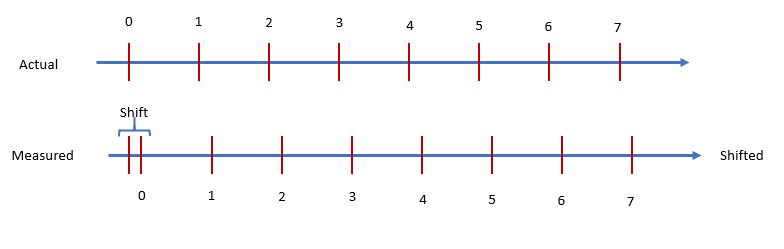
When distance \(d_{\mathcal{E}}=0\), distance \(d_{\mathcal{P}} > 0\). This causes a shift in what is observed at infinity to what is physically happening. Zero is observed when a magnitude or \(r\) is still greater than zero. This makes a type of discreteness-discontinuity at zero, a type of shift as shown in Figure below. Calculus is not an option when working with discrete spaces, and neither are Riemannian manifolds. Thus, the ability to transfer between spherical surfaces needs a solution that is not continuous. A method to approximate with the ability to scale to a high level of precision is sought. For clarity and completeness, the transformation does not create a pure numerical discreteness. Instead, it creates a shifted zero quantity (\(0_{shifted}=Constant \geq 0\)); thus, every number on a number line is shifted by observation. However, the underlying forces must be calculated using the un-shifted values. Consider a transformation of a radial distance:
\begin{equation}
r’=(1+\frac{k}{r})r = r + k
\end{equation}
Where \(k\) is a constant. When \(r=0\), \(r’\) is not zero. Thus, any \(\Delta r\) between spherical radial lengths is:
\begin{equation}
\Delta r = \Delta r + k
\end{equation}
To an observer, the \(k\) value is not measured since they started at zero with no gaps (it was considered smooth when they measured the difference), but the physical laws behave with the \(k\) value included. Contemplate a center potential energy calculated as
\begin{equation}
E=\frac{1}{r}
\end{equation}
as measured by an observer, but hidden to the observer is the shift in zero as in the figure below thus what is measured is
\begin{equation}
E=\frac{1}{r+k}
\end{equation}
When a \(\Delta E\) is calculated, it is not
\begin{equation}\label{eqE1}
\Delta E=\frac{1}{r_{final}}-\frac{1}{r_{initial}}
\end{equation}
but instead, it is
\begin{equation}\label{eqE2}
\Delta E=\frac{1}{r_{final}+k}-\frac{1}{r_{initial}+k}
\end{equation}
When \(r \gg k\), the difference is not measurable, but as \(r\) approaches \(k\) in magnitude, the measurements will show a considerable difference. Second, if there is a summation over spherical surfaces of differing \(r\) magnitudes, the \(k\) value may become a multiplier effect. In the theory’s transformation, a radial orbit could be observed as zero magnitude, yet the observed center-based force would not be zero.
The theory, at this juncture, predicts when observing the large (\(r>>0\)), there is a negligible (possibly not even measurable) effect when considering a smooth manifold. But as \(r \rightarrow 0\) there may be conflicting observations to physical laws like a \(\frac{1}{r}\) based force, where a zero radius produces a force. It should be noted in Schwartzschild’s solution to Einstein’s equation the metric
\begin{equation}
\begin{split}
c^{2}d\tau^{2}=\left(1-\frac{2GM}{rc^{2}}\right)c^{2}\mathit{dt} \
-\left(1-\frac{2GM}{rc^{2}}\right)^{-1}dr^{2}-r^{2}\left(d\theta^{2}+\sin^{2}\theta d\varphi^{2}\right)
\end{split}
\end{equation}
is used. When transforming the length \( c^{2}d\tau^{2}\) as observed from infinity to a local observer’s position within the gravity well, the metric reduces to:
\begin{equation}
c^{2}d\tau^{2}=-\left(1-\frac{2GM}{rc^{2}}\right)^{-1}dr^{2}
\end{equation}
By performing a series expansion about \(\frac{M}{r}\)
\begin{equation} \label{eqGRseries}
\begin{split}
\left(1-\frac{2GM}{rc^{2}}\right)^{-\frac{1}{2}}dr \
= \left( 1+\frac{GM}{rc^{2}}+\frac{3G^{2}M^{2}}{{2r^{2}c}^{4}} +\mathrm{O}\left(\left(\frac{M}{r}\right)^{3}\right) \right) dr
\end{split}
\end{equation}
and observing when \(dr = r\), a constant in the series emerges.
\begin{equation}\label{eq14}
\frac{2 G M}{c^2}
\end{equation}
This is the same as NUVO’s static zero value. It appears GR has the same number line shift built into it. As \(r \rightarrow dr^2\) the \(r\) in \((\frac{G M}{r c^2})\) cancels leaving the constant value.
It is here the author contends the theory’s transformation corresponds to GR when \(r>>0\) and only the static field is considered (no motion in the field). At values of \(r\) where \(r>>0\), the theory’s number line shift has less and less impact, allowing the treatment of a smooth manifold in these areas to produce small effects (possibly immeasurable errors compared to empirical data). But unlike GR, NUVO reflects the constant (the shift in the observable number line) and exploits this feature to form a possible seamless path to a unified theory.
Having shown that a manifold approach does not work for the theory, the next starting point is to consider a transformation from one frame (coordinate system) to another. This is not straightforward, as there are, at minimum, two types of transformations: static and dynamic.